Ground Pentrating Radar Case Study:
Ground Penetrating Radar (GPR) is a high frequency EM technique used to image the earth at shallow depths but with high resolution. This technique is often used to map stratigraphy, locate voids, map utility cables, and detect buried waste and even dead bodies. The method uses two antennas: one to transmit a continuous EM signal and a second to measure the response. Once the effect of the transmitter antenna (Tx) is subtracted from the receiver (Rx) response, any remaining signal must be caused by objects in the earth reflecting and scattering the transmitted wave.
In most cases, the geophysicist looks at the reflection and scatter pattern from the buried objects and tries to determine what objects caused the response. As part of my Master's thesis, I wrote a computer imaging algorithm to processed the reflected and scattered energy and create an image of the object that caused the response. The algorithm solves for any objects in the earth and records them as velocity values. Good conductors have low velocity values and resistors have high velocity values. I wrote the algorithm to process data in two dimensions (if just a line of data were collected) and in three dimensions (if a grid of data were collected). The intent of the algorithm was to make the interpretation of the data much easier for the geophysicist.
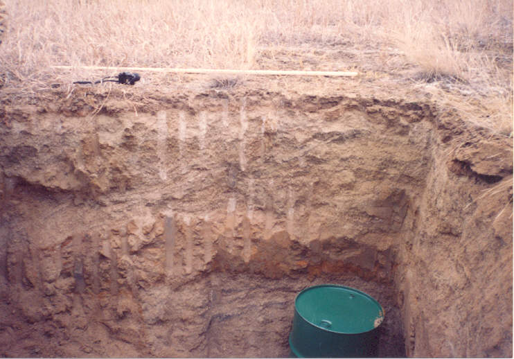
To test the effectiveness of the algorithm, my adviser and I constructed a test site. We buried three empty 55 gallon drums in a pit and carefully measured the positions and dimensions of the drums and the location of the pit walls (Figure 1). The pit was dug in sandy alluvial material with disseminated clays and black magnetite sands present. Two of the drums were metal and one was plastic. Later that year, we returned to the site to survey the area using GPR. The test site was examined using a 41 by 41 grid of stations with a 0.30 meter separation between stations and a 0.61 meter offset between Tx and Rx (Figure 2).
Figure 1: The placement of a barrel in the pit is shown. A clay layer can be seen immediately above the barrel.

Figure 2: Line 24 goes directly over the standing metal drum and the laying down plastic drum.
Figure 3 shows the raw data record for profile line 24 located directly over the standing metal and horizontal plastic barrels. The raw record is displayed in a format called a shaded wiggle trace plot. The horizontal axis is the position of the midpoint between the Tx and Rx and the vertical axis is time. Since more time is required for the transmitter wave to travel deeper and be reflected back to the surface, the time axis is proportional to depth. The amplitude of the response is represented by a wiggle trace when positive responses are shaded in black. The scattering response from the metal barrel is apparent by the hyperbolic curve with its peak located at station 16 and 28 nanoseconds. It is difficult to see any scattering response from the plastic barrel.

Figure 3: Schematic drawing indicates barrel locations in the pit for Line 24. Raw wiggle trace plot of the profile is shown below. The time window matches the depth cross section for a background velocity of 0.11 m/ns.
Figure 4 shows the results of processing the 2-D and 3-D processed data for profile line 24. The low velocity anomaly at station 16 and depth of 1.5 meters corresponds with the top of the upright barrel. The high velocity anomaly at station 21 and depth of 1.2 meters corresponds to the center of the plastic barrel. The 2-D and 3-D methods both successfully indicate the barrel locations. The 3-D procedure increases the strength of the anomalies and indicates a multiple of the primary diffraction from the metal drum. The 3-D algorithm is also better at defining the edge of the pit walls. There are continuous high velocity bands in the earth that correspond to the depths of the clay layers. These bands are abruptly discontinued at the pit boundaries where they were disrupted by the process of digging the pit. Finally, Figure 5 shows a three dimensional image of the pit. Two fences showing the GPR response along two of the pit walls are shown. The highest and lowest velocity areas are represented by solid red and blue shapes, respectively. The largest of these anomalies are caused by the three barrels, but there are a few low and high velocity anomalies outside of the pit which are probably caused by clay concentrations.

Figure 4: Cross sections of 2-D (a) and 3-D (b) processing of the raw data shown in Figure 3. the background velocity is 0.11 m/ns. Low (high) velocities are indicated by dark (light) colors.

Figure 5: 3-D image of the three drums in the pit. Fence diagram lines are added on two sides of the pit to show the GPR response from the background earth.
Ground penetrating radar is a useful technique for high resolution imaging of the near surface earth. Numerous processing techniques are available for improving these images. Whenever I use GPR for a project, I carefully select which processing enhancing and imaging techniques I use for the best results possible.